In the realm of computer science and programming, the efficiency of algorithms plays a pivotal role in determining the performance of software applications. How do we quantify and compare the efficiency of different algorithms, especially when faced with varying input sizes?

Enter **Big O notation**, a powerful tool that allows developers to express the scalability and efficiency of algorithms in a language-independent manner. Whether you're a budding programmer or an experienced developer, understanding Big O notation is crucial for writing efficient and scalable code.

What is Big O Notation?

At its core, Big O notation provides a way to describe the time and space complexity of an algorithm concerning the size of its input. It enables developers to analyze and compare the efficiency of algorithms, helping them make informed decisions when selecting the right solution for a given problem.

The Basics in Simple Terms

Let's break down Big O notation into simple terms:

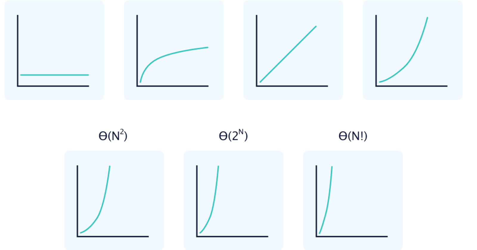
1. Constant Time (O(1)):

• An algorithm with constant time complexity has a consistent execution time, regardless of the input size. Imagine fetching the first element from an array; it takes the same amount of time, no matter how large the array is.

2. Linear Time (O(n)):

- Linear time complexity signifies that the execution time grows linearly with the size of the input. As we iterate through each element in an array, the time taken increases proportionally with the array's size.

3. Quadratic Time (O(n^2)):

- Quadratic time complexity indicates a significant increase in execution time as the input size grows. Nested loops iterating over an array exemplify this scenario, making it a less efficient choice for large datasets.

4. Logarithmic Time (O(log n)):

- Logarithmic time complexity, often seen in binary search algorithms, implies that the execution time grows slowly as the input size increases. It's a more efficient choice for handling large datasets compared to quadratic time complexity.

Bridging Theory and Practice: Code Examples

To solidify our understanding, let's delve into some practical examples:

Example 1: Constant Time

function printFirstElement(array) {

console.log(array[0]);

}

In this function, regardless of the array's size, fetching and printing the first element takes constant time.

Example 2: Linear Time

function printAllElements(array) {

for (let i = 0; i < array.length; i++) {

console.log(array[i]);

}

}

As we iterate through each element in the array, the execution time grows linearly with the array's size.

Example 3: Logarithmic Time

function binarySearch(sortedArray, target) {

let low = 0;

let high = sortedArray.length - 1;

while (low <= high) {

const mid = Math.floor((low + high) / 2);

const guess = sortedArray[mid];

if (guess === target) {

return mid; // Found the target

} else if (guess > target) {

high = mid - 1; // Adjust the search range

} else {

low = mid + 1; // Adjust the search range

}

}

return -1; // Target not found

}

Binary search is an example of logarithmic time complexity, making it efficient for searching in large datasets.

Conclusion

Big O notation is a fundamental concept that empowers developers to make informed decisions about algorithm selection based on the efficiency required for a given task. As you embark on your coding journey, keep honing your understanding of Big O notation, practice analyzing algorithmic complexities, and watch as your ability to craft efficient, scalable code grows.

Stay tuned for more in-depth explorations of advanced Big O complexities and real-world applications in upcoming blog posts!